02 - Metric Taxonomy

This is the first pass of a decision-grade metric set for action-conditioned world models. Each metric is chosen because it answers a question an applied team would actually ask before integrating a model.

What “decision-grade” means here

A metric is decision-grade when both of the following hold:

1. Its units translate directly to a deployment-time cost or capability. Success rate is a fraction in [0, 1]. Planning latency is in milliseconds. Compute per decision is in policy-declared units (FLOPs, model forward passes, rollouts). Perturbation recovery is a fraction. All of these are quantities a procurement, robotics, or controls team can act on without further conversion.

2. It is computable from a closed-loop run of the model, not from the model in isolation. Reconstruction loss, FID, next-frame prediction error, and embedding-distance benchmarks are model-internal quantities - they describe how well the model fits its training distribution. A decision-grade metric requires the model to be used (encoded, rolled out, scored, planned) inside an environment, and reports what happened to the agent as a result.

The two criteria together exclude both pure prediction quality (which fails criterion 2) and abstract “alignment” or “interpretability” scores that do not translate into shippable units (which fail criterion 1).

The taxonomy below lists the metrics that meet both criteria in this study’s first pass. Additions are welcome; the contribution procedure in CONTRIBUTING.md requires every proposed metric to pass the same two-criterion test.

Summary table

Hover (or focus) any metric name to see its formula in a popover. The popover is the canonical definition; this page does not duplicate the formulas anywhere else.

Metric	Definition	Why it matters	Example measurement
Action Success Rate Reads as: how often did the agent reach the goal? $$\text{success\_rate} \;=\; \frac{\text{episodes that succeeded}}{\text{episodes total}}$$ Bounded in $[0, 1]$. If this is near zero, no other metric matters.	Fraction of episodes in which the agent reaches the goal within the horizon.	The headline number. If this is near zero, nothing else matters.	Over 200 episodes of Two-Room with horizon 50, success rate = 0.87.
Planning Latency Reads as: how long does a single plan() call take, on average? $$\bar{\ell} \;=\; \frac{\text{total ms spent in plan()}}{\text{total number of plan() calls}}$$ Per call, not per episode. A policy that replans more often cannot hide behind a per-episode mean.	Wall-clock time to produce one planned action sequence. Reported per plan() call, not per episode.	Tells you whether the model can close a control loop in real time.	mean = 2.4 ms per plan() call on the maze toy (CPU).
Compute per Decision Reads as: how much model work, in policy-declared units, does one executed action take? $$\bar{c} \;=\; \frac{c_{\text{plan}} \;\times\; \text{total plan() calls}}{\text{total executed steps}}$$ For TabularWorldModelPlanner: $c_{\text{plan}} = N_{\text{cand}} \cdot H_{\text{plan}}$ rollout-units.	Estimated FLOPs or model forward passes per planned action.	Translates research compute into product cost (energy, dollars, GPU hours).	1.2 model rollouts per decision, average horizon 8.
Planning Horizon Reads as: smallest lookahead beyond which a deeper search does not buy meaningfully more success. $$H^{\ast} \;=\; \min\Bigl\{\,H \,:\; \text{success}(H') - \text{success}(H) \leq \epsilon \;\;\forall\, H' > H\,\Bigr\}$$ For the maze toy with $\epsilon = 0.01$: $H^{\ast} = 15$, one step past the maze's optimal-path length.	Effective look-ahead depth at which performance stops improving.	Tells you how far the model can usefully imagine before it becomes noise.	Success rate plateaus at horizon = 12; longer horizons add cost without value.
Perturbation Recovery Reads as: of episodes where env.perturb() actually fired, the fraction that still reached the goal. $$r \;=\; \frac{\text{actually-perturbed episodes that succeeded}}{\text{actually-perturbed episodes}}$$ "Actually-perturbed" excludes episodes that succeed before the perturbation step (v0.3.1 fix).	Success rate conditional on a perturbation event during the episode.	Measures robustness in the only way a real environment delivers it - by surprise.	Baseline success = 0.87; under perturbation = 0.61; recovery rate = 0.70.
Sample Efficiency Reads as: performance as a function of training samples or environment interactions. No single closed-form formula. Reported as the sample count at which the model reaches a fixed fraction (typically 0.8) of its asymptotic success rate. Track the success-rate-vs-samples curve.	Performance as a function of training samples or environment interactions.	Distinguishes models that need a research-lab dataset from models that can ship.	Reaches 80 percent of asymptotic success with 5k transitions.
Surprise Detection Reads as: how well does the model flag out-of-distribution inputs? $$\text{AUROC} \;=\; \Pr\!\bigl[\,\text{score}(\text{anomalous}) \,>\, \text{score}(\text{in-distribution})\,\bigr]$$ $0.5$ is random ranking, $1.0$ is perfect. score is a model-defined surprise signal (negative log-likelihood, distance from latent prior, etc.).	Ability of the model to flag observations its predictor finds unlikely.	A precondition for safe behaviour - "I do not know what is going on" is a feature.	AUROC = 0.78 on held-out anomalous frames vs in-distribution frames.
Latent Interpretability Reads as: does the latent state expose task-relevant structure? $$R^{2} \;=\; 1 \;-\; \frac{\sum_{i}(y_i - \hat{y}_i)^2}{\sum_{i}(y_i - \bar{y})^2}$$ Typically reported as the $R^{2}$ of a linear probe predicting a task-relevant variable (agent position, object pose) from the latent. Very high values may indicate the latent is just the input.	Degree to which the latent state exposes task-relevant structure.	Helps debugging, safety review, and integration with classical control.	Linear probe on latent predicts agent position with $R^2 = 0.93$.
Wilson 95% interval Reads as: lower and upper bounds for the success rate, defendable at 95% confidence. Asymmetric near 0% and 100% (which is where horizon sweeps spend most of their data). $$\hat{p}_{\text{lo}}, \hat{p}_{\text{hi}} \;=\; \frac{\hat{p} + \dfrac{z^{2}}{2n} \;\pm\; z\sqrt{\dfrac{\hat{p}(1-\hat{p})}{n} + \dfrac{z^{2}}{4n^{2}}}}{1 + \dfrac{z^{2}}{n}}$$ $z = 1.96$ for two-sided 95%. At $\hat{p} = 1$, $n = 30$: $[0.89, 1.00]$. To push the lower bound to $0.95$ at the same $\hat{p}$: $n \geq 73$.	Lower and upper bounds for the observed success rate, asymmetric near the extremes.	Tells you what reliability you can defend to a procurement or regulatory team, not just the point estimate.	$\hat{p} = 1.00$ over $n = 30$ gives $[0.89, 1.00]$ at 95% confidence.
Normal CI on mean latency Reads as: the range around the observed mean latency where 95% of constructed intervals would contain the true mean. $$\bar{\ell} \;\pm\; 1.96 \cdot \frac{\sigma_{\ell}}{\sqrt{n_{\ell}}}$$ $\sigma_{\ell}$ is the standard deviation of the per-call latencies; $n_{\ell}$ is the total number of plan() calls across all episodes.	Symmetric interval on the mean per-call latency.	Normal works here because latencies are bounded away from 0 and we typically have many samples.	$\bar{\ell} = 2.35 \pm 0.05$ ms per call on the maze toy at horizon 15.
Counterfactual Planning Gap (CPG) Reads as: the success-rate cost of using a learned model instead of the oracle in the same planner. $$\mathrm{CPG} \;=\; \mathrm{success\_rate}(\mathrm{oracle}) \;-\; \mathrm{success\_rate}(\mathrm{learned})$$ Both planners share env, episodes, seed, horizon, and score function. Only the dynamics callable changes. The 95% CI uses the Agresti-Caffo plus-4 adjustment, which keeps the variance positive at $p \in \{0, 1\}$ and gives honest coverage for small $n$. The cpg_verdict() branch is gated on the AC lower bound, not on the raw point estimate, so a noisy $+0.10$ gap from $n=10$ correctly reports INCONCLUSIVE rather than MODEL BOTTLENECK. See wmel.metrics.CPGResult and cpg_verdict.	Success-rate gap between an oracle-dynamics planner and the same planner using a learned model. Packaged as a single scalar with an Agresti-Caffo CI and a gated verdict.	Decomposes model error from planner capacity. The packaged-scalar form (with CI and gated verdict) is new in this framework; the underlying oracle-vs-learned-rollout comparison is in the spirit of model-exploitation analyses in MOPO and MOReL.	On DMC Acrobot-swingup with random-shooting MPC, 10 episodes each: raw $\mathrm{CPG} = +0.30$, AC 95% CI $[-0.06, +0.56]$ (crosses zero). Verdict: INCONCLUSIVE at $n=10$ - suggestive of a model bottleneck but more episodes are needed to confirm.

Planning-horizon curve (worked example)

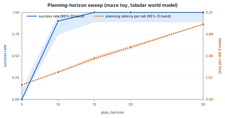
The “Planning Horizon” metric is operationalised by wmel.experiments.horizon_sweep. Running it on the maze toy environment with TabularWorldModelPlanner produces a textbook curve - per-call planning latency grows monotonically with horizon, success rate plateaus, and beyond the plateau steps-to-success starts to degrade because the planner over-commits before replanning:

Horizon sweep: tabular-world-model
  plan_h |   success |          95% CI |   steps | latency_ms |       95% CI (ms)
  -------------------------------------------------------------------------------
       5 |     0.000 | [0.00, 0.11]   |     n/a |      0.882 | [0.87, 0.89]
      10 |     0.900 | [0.74, 0.97]   |    31.3 |      1.588 | [1.56, 1.62]
      15 |     1.000 | [0.89, 1.00]   |    30.5 |      2.393 | [2.34, 2.44]
      20 |     1.000 | [0.89, 1.00]   |    33.8 |      3.085 | [3.08, 3.09]
      30 |     1.000 | [0.89, 1.00]   |    41.8 |      4.579 | [4.55, 4.60]

Reading the curve:

• plan_h=5 is too shallow to find a solution. Success is 0 percent.
• plan_h=10 mostly works (90 percent success) but is brittle.
• plan_h=15 matches the maze’s optimal path length and saturates at 100 percent.
• Past the plateau, latency keeps rising while success does not move and steps-to-success degrades - a clean illustration of the “useful look-ahead depth” the metric is meant to expose.

Latency is measured per plan() call (the unit the metric is defined in), not per episode. Replanning more often does not earn a policy a free latency discount. The success-rate column uses a Wilson score interval; the latency column uses a normal interval on the sample mean. The same script writes the full report as JSON to examples/maze_toy/horizon_sweep_report.json for downstream tooling.

Reproduce with:

python -m examples.maze_toy.run_horizon_sweep

Paste-ready Markdown

wmel.experiments.to_markdown_horizon_sweep(sweep) returns the same data as a Markdown table - including the compute-per-decision column - that drops directly into a PR description or a doc:

### Horizon sweep: `tabular-world-model`

| plan_horizon | success_rate | success_95ci | avg_steps | latency_ms_per_call | latency_95ci | compute_per_decision |
| ---: | ---: | :--- | ---: | ---: | :--- | ---: |
| 5 | 0.000 | [0.00, 0.11] | n/a | 0.875 | [0.87, 0.89] | 368.250 |
| 10 | 0.900 | [0.74, 0.97] | 31.3 | 1.578 | [1.55, 1.61] | 350.575 |
| 15 | 1.000 | [0.89, 1.00] | 30.5 | 2.348 | [2.34, 2.36] | 278.689 |
| 20 | 1.000 | [0.89, 1.00] | 33.8 | 3.096 | [3.07, 3.12] | 256.410 |
| 30 | 1.000 | [0.89, 1.00] | 41.8 | 4.614 | [4.55, 4.68] | 277.512 |

The three metric dimensions - planning horizon, latency per call, and compute per decision - now appear together on one row, which is the trade-off surface this taxonomy advocates.

wmel.report.to_markdown_scorecard(scorecard) does the same for a single scorecard.

Notes

• Latency, compute, and horizon form a single trade-off surface. A useful scorecard reports them together, not in isolation.
• Perturbation Recovery requires a perturbation library. wmel.perturbations ships three composable types: EnvPerturbation (delegates to env.perturb()), DropNextActions(k) (action-level - simulates actuator drops by removing the next k queued actions), and CompositePerturbation(*parts) (chains the first two for combined failure modes). BenchmarkRunner takes a perturbation kwarg and records the chosen strategy on the Scorecard, so a policy benchmarked under different perturbations produces distinguishable scorecards.
• Surprise Detection and Latent Interpretability are model-level diagnostics. They are part of the scorecard because they are precisely what a research-grade predictor is supposed to be good at - if it is not, that is itself a finding.
• All metrics should be reported with seeds, sample sizes, and confidence intervals when feasible.

Versioning

This taxonomy is intentionally a starting point. Additions are welcome, but every new metric should answer an applied question, come with an example measurement, and have a corresponding test on synthetic data.