
Random
Samples actions uniformly at random.
0%
success rate over 30 episodes
- latency / call
- 0.03 ms
- compute / decision
- n/a
- verdict
- Wanders near the start. Goal stays out of reach.
Note on this page vs. the paper (v0.18)
The paper reports the authoritative task-level results: each episode samples the task's initial-state distribution (the two CPG arms paired by start state), which is what makes the heterogeneous verdicts above. The Step-04 walkthrough below opens with the original single-fixed-initial-state Acrobot example, then shows the metric correcting itself: sampling the task distribution collapses the oracle there and overturns the verdict (the paper's self-correction section).
Static AI benchmarks measure how well a model predicts. They miss what an applied team actually needs to know: success rate, latency budget, compute cost, robustness under perturbation. This is a small, opinionated evaluation layer that closes that gap.
The next bottleneck for world models is not only model quality. It is proof of usefulness.


Step 01
Action-conditioned world models are routinely evaluated on prediction quality: reconstruction loss, FID, held-out next-frame accuracy. None of these answer the question an applied team must answer before integrating a model into a control loop.
The question is decision quality, not prediction quality. Does the model, when used by a planner, produce decisions that succeed within the latency and compute budget the deployment will accept? Does it recover from perturbations? Does it generalise across related tasks?
A low validation MSE is necessary but not sufficient. The framework’s headline example: a Markovian MLP world model with val_mse $= 0.026$ on DMC Acrobot. Predicting accurately. Planning a $0\%$ success rate.
See Thesis and Evaluation gap for the long form.
Step 02
Every adapter exposes four hooks. The benchmark runner does the rest: rollouts, perturbations, latency measurement, scorecard.

The contract is intentionally minimal: encode (observation → latent), rollout (latent + action sequence → latent sequence), score (latent + goal → reward), plan (observation + goal + horizon → action sequence). Anything that implements these four methods plugs into the same runner and gets compared on the same scorecard structure.
Concrete subclasses live in src/wmel/adapters/: a stdlib tabular planner, a PyTorch MLP, and the DMC Acrobot oracle. None of them know about the runner, the metrics, or each other.
Step 03
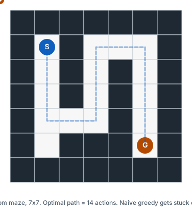
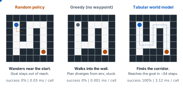
A 7x7 maze with a vertical wall and one doorway. Same env, same 30 episodes, same seed; three different planners. The framework's first non-trivial demonstration that the contract holds and the metrics discriminate.
Samples actions uniformly at random.
success rate over 30 episodes
Always step toward the goal in Manhattan distance.
success rate over 30 episodes
Random-shooting MPC over a learned-style dynamics function.
success rate over 30 episodes
The thesis is only credible if a real learned model can plug into the same evaluation layer. The smallest demonstration: a tiny PyTorch MLP trained on 64 maze transitions, passed in as the dynamics= callable.
The reference run from the section above.
success rate over 30 episodes
Same MPC planner, dynamics is now a tiny MLP trained on 64 transitions.
success rate over 30 episodes
Same success, same steps to success, same nominal compute – 76 times the per-call latency at horizon 20. Without measuring latency per call, you would conclude “it works just as well!” while the actual deployment cost is two orders of magnitude higher.
Sweep the planning horizon of the tabular world-model planner and watch where it pays off. Hover any horizon to see all four metrics together. Success saturates at $h = 15$; per-call latency keeps climbing past the plateau without buying any extra success.
Step 04
The framework's flagship metric. Run the same random-shooting MPC planner twice on DeepMind Control Suite Acrobot-swingup — once against oracle dynamics (real MuJoCo physics), once against a Markovian MLP world model trained on 2 000 random transitions. The only thing that changes is the dynamics= callable. The success-rate difference is the Counterfactual Planning Gap.
Random-shooting MPC against real MuJoCo physics.
success rate over 10 episodes
Same MPC, same scoring, MLP trained on 2 000 random transitions.
success rate over 10 episodes
Decoupling model error from planner capacity.
raw difference of success rates
A low validation MSE on prediction quality does not translate into closed-loop success. CPG quantifies the planning-side gap with an Agresti–Caffo $95\%$ confidence interval that does not collapse at the boundary proportions $p \in {0, 1}$ where the standard Wald approximation degenerates. The verdict is gated on the CI lower bound, not the raw point estimate – at $n = 10$ the framework reports INCONCLUSIVE rather than over-claiming a model bottleneck.
That INCONCLUSIVE at $n = 10$ is suggestive, so the natural next step is more episodes. Pooling three seeds and switching to a stronger CEM planner makes the gap look decisive: the oracle solves $88\%$ of episodes, the learned arm stays at zero, and the verdict hardens to MODEL BOTTLENECK ($\mathrm{CPG} = +0.88$, AC CI $[+0.81, +0.92]$). A point-estimate leaderboard would publish that headline.
It is an artifact. Every one of those episodes started from the same fixed initial state – a deterministic env reset, with only the planner’s internal randomness varying – and on Acrobot that start happens to be an unusually easy swing-up. Sampling the task’s actual initial-state distribution (a fresh start per episode, the two arms paired by start state) collapses the oracle’s success rate from $0.88$ to $\sim!3\%$. With the oracle planner itself solving only $\sim!3\%$ of random starts, the gap closes and the verdict flips to PLANNER BOTTLENECK: even a perfect model would not help, because the search cannot solve the task from a typical start.
| Initial state | Planner | Dynamics | Oracle | Learned | CPG (AC 95% CI), verdict |
|---|---|---|---|---|---|
| fixed, pooled 150 | CEM | TD-MPC2 | $0.88$ | $0.00$ | $+0.88$ $[+0.81, +0.92]$, MODEL BOTTLENECK |
| task, pooled 150 | CEM | MLP | $0.033$ | $0.020$ | $+0.013$ $[-0.027, +0.053]$, PLANNER BOTTLENECK |
| task, pooled 150 | CEM | TD-MPC2 | $0.033$ | $0.027$ | $+0.007$ $[-0.035, +0.049]$, PLANNER BOTTLENECK |
This is the single strongest piece of evidence for what the metric is for: a calibrated, interval-gated statistic, run honestly over the task distribution, overturned a headline that a point estimate at one configuration would have published. The prediction-vs-decision dissociation still holds – the learned MLP’s held-out validation MSE is low while its planning success is zero – but the load-bearing diagnosis is now about the planner and the distribution, not the model.
Read the full page on CPG → · Read the paper →
Run over the task distribution on all three DeepMind Control Suite tasks, the verdict is heterogeneous – the gate fires four of its five branches on real data, which is precisely what a calibrated metric should surface and what a point-estimate leaderboard cannot.
PLANNER BOTTLENECK (above): the oracle planner itself solves only $\sim!3\%$ of random starts, so neither arm wins.MODEL BOTTLENECK in all four cells. The oracle solves the reach perfectly ($1.000$), both learned arms are clearly non-zero ($0.667$ to $0.800$), and yet every AC lower bound on the gap ($\mathrm{CPG}$ $+0.20$ to $+0.33$) stays strictly positive. The verdict tracks gap magnitude, not just a learned arm pinned at zero.LEARNED OUTPERFORMS ORACLE: the learned model lets CEM solve $0.733$ of episodes against the oracle planner’s $0.467$, so $\mathrm{CPG} = -0.27$, with the AC CI $[-0.48, -0.02]$ and a paired-bootstrap CI $[-0.50, -0.03]$ both clearing zero. The other Cartpole cells are MODEL BOTTLENECK or INCONCLUSIVE – one environment, three branches.Because the verdict gate is a function of the confidence interval, it also answers a question a bare leaderboard cannot: how many episodes a comparison needs before its ranking is trustworthy. A plausible $0.94$-vs-$0.92$ near-tie at $n = 100$ is statistically indistinguishable from noise; the gate shows it needs $n = 209$ per arm before the interval clears zero.
Cross-env (Cartpole) → · Third env (Reacher) → · Power analysis →
Step 05
No GPU, no heavy ML dependency at runtime. Core install plus an installed CLI; optional extras for PyTorch and DMC.
git clone https://github.com/Denis-hamon/world-model-eval-lab.git
cd world-model-eval-lab
pip install -e ".[dev]"
Then run a single benchmark or sweep the planning horizon via the installed wmel console script:
# One scorecard, one JSON report
wmel run --env maze_toy --policy tabular-world-model --episodes 30 --output run.json

# Horizon sweep, comma-separated horizons, one combined JSON
wmel sweep --env maze_toy --plan-horizons 5,10,15,20,30 --output sweep.json
The DMC Acrobot CPG worked example needs the [control] and [learned] extras:
pip install -e ".[dev,control,learned]"
python -m experiments.dmc_acrobot.cpg
# -> results/dmc_acrobot/cpg.json
Every JSON report carries a versioned envelope (schema_version, wmel_version, generated_at).
For the researcher
The metric taxonomy, the four-method evaluation contract, and the CPG definition with its Agresti-Caffo CI and gated verdict.
For the practitioner
A walkthrough of one scorecard, the benchmark cards each environment maps to, and the industrial use-cases the framework is built around.
For the reader
The short paper accompanying the framework, the LaTeX source, the reproducibility script, and the citation entry.
Tagged GitHub releases run through v0.11.0 (the framework and the first paper draft). The research milestones since then are tracked in the paper and the version number; a consolidated v1 release will be tagged when the paper is submitted. Version labels below link to their release tag where one exists, otherwise to the paper section that documents the milestone.
Task-level rewrite: heterogeneous verdicts and a self-correction
The paper is rewritten on task-level results -- each worked example samples the task's initial-state distribution (arms paired by start state), produced by the opt-in --varied-init harness (experiments/_seeding.py, RERUN_VARIED_INIT.md; default off, so the original fixed-init results still reproduce). The verdict is heterogeneous: Acrobot flips to PLANNER BOTTLENECK (oracle solves ~3% of random starts -- the fixed-start MODEL BOTTLENECK was an artifact), Reacher holds MODEL BOTTLENECK, and high-capacity Cartpole under CEM reaches LEARNED OUTPERFORMS ORACLE ($\mathrm{CPG} = -0.27$, AC + paired-bootstrap CIs clear zero). Four of the five verdict branches fire on real data. Adds a paired-bootstrap CI and value-equivalence citations. No new git tag.
Third environment: DMC Reacher-easy
The four-arm CPG matrix replayed on a third env: the first task with a two-dimensional action and an exactly-reconstructed oracle. Oracle solves the reach in every cell ($1.000$); both learned arms are clearly non-zero (TD-MPC2 $0.567$–$0.633$, the paper's highest), so all four cells are MODEL BOTTLENECK on non-degenerate gaps at the evaluated fixed initial state ($+0.367$ to $+0.700$) — the cleanest evidence the metric tracks gap magnitude, not just presence. The varying-initial-state re-run that supersedes these fixed-init numbers landed in v0.18. See the paper's Reacher section; Figure 3 extended to three series.
Power analysis: how many episodes a ranking needs
The verdict gate, read as a power calculator: ac_ci_half_width, required_n_for_half_width, detectable_gap_at_n. A plausible $0.94$-vs-$0.92$ leaderboard near-tie at $n = 100$ is shown statistically indistinguishable from noise (needs $n = 209$). Paper power-analysis section + Figure 5. Also: CPG positioned neutrally against the concurrent swm platform paper.
Cross-environment: DMC Cartpole-swingup, two capacities
Four-arm CPG matrix on a second env at TD-MPC2 model_size = 5 AND model_size = 1, $n = 30$ pooled each. At this fixed-init stage all four cells at size = 5 read MODEL BOTTLENECK and the CEM×TD-MPC2 cell at size = 1 flips to INCONCLUSIVE (learned $0.533$ vs oracle $0.500$, CPG $-0.033$, CI $[-0.28, +0.21]$). The v0.18 task-level re-run supersedes these numbers: the size-5 CEM×TD-MPC2 cell becomes LEARNED OUTPERFORMS ORACLE ($\mathrm{CPG} = -0.27$). See the paper's cross-environment section + Figures 3 and 4.
First two paper figures (CPG vs data, coverage histogram)
PGF/TikZ Figure 1 (val MSE plummets $\sim 150\times$ while CPG stays flat at $+0.267$, asymmetric Agresti-Caffo CI) and Figure 2 (uprightness coverage: $0/2000$ random states reach upright vs $20.2\%$ for oracle). Two adversarial-review fixes addressed: sig-fig parity and asymmetric error bars.
Robustness sweep: published model, stronger planner, perturbation
Three new axes test the v0.11 MODEL BOTTLENECK verdict: TD-MPC2 (2M env steps) as dynamics, CEM as planner, DropNextActions(k) as in-episode perturbation. Verdict survives all three; pooled-150 under CEM tightens CI half-width to 0.054. See the paper's robustness sections.
Multi-seed CPG sweep: capacity vs.\ coverage
Verdict hardens from INCONCLUSIVE (n = 10) to MODEL BOTTLENECK (n = 150 pooled across three seeds); training-set sweep across {200, 2 000, 20 000} transitions leaves verdict and CI identical while validation MSE drops 150×. Paper Section 5.5 + 5.6 updated.
Short paper: Counterfactual Planning Gap
~7-page LaTeX paper under paper/, 23 BibTeX entries, reproducibility script, three adversarial-review findings addressed before tag.
CPG metric with Agresti-Caffo CI and gated verdict
Five-branch verdict gated on the CI lower bound; honest INCONCLUSIVE at n=10 instead of over-claiming a Wald-CI-driven significance.
DMC Acrobot-swingup wired in
First non-toy environment via wmel.envs.dmc_acrobot, with a Markovian MLP learned dynamics and an oracle dynamics factory. dm-control is an optional extra.
CLI, versioned JSON schema, perturbation-aware sweep
wmel run / wmel sweep console scripts; JSON envelope with schema_version, wmel_version, generated_at. Second CI job locks the no-torch runtime promise.
Proof of contract for learned PyTorch dynamics
PyTorch MLP fits the maze's transition table and plugs in as a drop-in dynamics= callable. Identical success, 76x higher per-call latency -- the trade-off the framework is built to expose.
Pluggable perturbation library
Perturbation, EnvPerturbation, DropNextActions, CompositePerturbation. Runner inner loop switched to deque for O(1) action-queue pops.
This is an independent study of evaluation methodology for action-conditioned world models. It is not an official artifact of AMI, Meta, the LeWorldModel project, or any of their authors, and not an artifact of any current or past employer of the author. References to JEPA-style or LeWorldModel concepts are conceptual, not affiliational.